This is the second in a short series on what package developers can do to reduce the latency of Julia packages. In the first post, we introduced precompilation and some of its constraints. We also pointed out that precompilation is closely tied to type inference:
precompilation allows you to cache the results of type inference, thus saving time when you start using methods defined in the package
caching becomes more effective when a higher proportion of calls are made with inferable argument types (i.e., type-inference "succeeds"). Successful inference introduces links, in the form of
MethodInstancebackedges, that permit the entire call graph to be cached.
As a consequence, anyone interested in precompilation needs to pay attention to type inference: how much time does it account for, where is it spending its time, and what can be done to improve caching? Julia itself provides the internal infrastructure needed to "spy" on inference, and the user-space utilities are in the SnoopCompile package. Julia 1.2 provided limited facilities for "spying" on inference, and this infrastructure corresponds to SnoopCompile's @snoopi macro. Julia 1.6 includes new changes that have permitted a far deeper look at what inference is doing. Appropriately enough, SnoopCompile calls this @snoopi_deep.
The rich data collected by @snoopi_deep are useful for several different purposes. In this post, we'll describe the basic tool and show how it can be used to profile inference. Later posts will show other ways to use the data to reduce the amount of type-inference or cache its results.
Collecting the data
To see @snoopi_deep in action, we'll use the following demo:
module SnoopDemo
    struct MyType{T} x::T end

    extract(y::MyType) = y.x

    function domath(x)
        y = x + x
        return y*x + 2*x + 5
    end

    dostuff(y) = domath(extract(y))

    function domath_with_mytype(x)
        y = MyType(x)
        return dostuff(y)
    end
end
The main call, domath_with_mytype, stores the input in a struct, and then calls functions that extract the field value and perform arithmetic on the result. To profile inference on this call, we simply do the following:
julia> using SnoopCompile

julia> tinf = @snoopi_deep SnoopDemo.domath_with_mytype(1)
InferenceTimingNode: 0.009382/0.010515 on InferenceFrameInfo for Core.Compiler.Timings.ROOT() with 1 direct childrenSnoopDemo module (by re-executing the command we used to define it) if you want to collect data with @snoopi_deep on the same code a second time. This won't redefine any Base methods that SnoopDemo depends on, so you still may see differences between running this in a fresh session and subsequent uses of @snoopi_deep.This may not look like much, but there's a wealth of information hidden inside tinf. While optional, before proceeding further it's recommended to check tinf for hints that invalidation may have influenced the result:
julia> staleinstances(tinf)
SnoopCompileCore.InferenceTiming[]
staleinstances extracts MethodInstances that have some "stale" generated code (code that is no longer callable). In our case, it returns an empty list, meaning that it found no stale instances, which guarantees that no invalidation occurred. There's nothing "funny" going on behind the scenes that will influence our results.
@snoopr, another macro exported by SnoopCompile, staleinstances does not distinguish between whether that stale code existed before you ran the @snoopi_deep block, or whether it got invalidated during the running of that block. For detailed analysis of invalidations, @snoopr is the recommended tool.Inspecting the output
In this post, we'll stick to the basics of inspecting the data collected by @snoopi_deep. First, notice that the output is an InferenceTimingNode: it's the root element of a tree of such nodes, all connected by caller-callee relationships. Indeed, this particular node is for Core.Compiler.Timings.ROOT(), a "dummy" node that is the root of all such trees.
You may have noticed that this ROOT node prints with two numbers. It will be easier to understand their meaning if we first display the whole tree. We can do that with the AbstractTrees package:
julia> using AbstractTrees

julia> print_tree(tinf)
InferenceTimingNode: 0.009382/0.010515 on InferenceFrameInfo for Core.Compiler.Timings.ROOT() with 1 direct children
└─ InferenceTimingNode: 0.000355/0.001133 on InferenceFrameInfo for Main.SnoopDemo.domath_with_mytype(::Int64) with 3 direct children
   ├─ InferenceTimingNode: 0.000122/0.000254 on InferenceFrameInfo for MyType(::Int64) with 1 direct children
   │  └─ InferenceTimingNode: 0.000132/0.000132 on InferenceFrameInfo for MyType{Int64}(::Int64) with 0 direct children
   ├─ InferenceTimingNode: 0.000071/0.000071 on InferenceFrameInfo for MyType(::Int64) with 0 direct children
   └─ InferenceTimingNode: 0.000122/0.000453 on InferenceFrameInfo for Main.SnoopDemo.dostuff(::MyType{Int64}) with 2 direct children
      ├─ InferenceTimingNode: 0.000083/0.000161 on InferenceFrameInfo for Main.SnoopDemo.extract(::MyType{Int64}) with 2 direct children
      │  ├─ InferenceTimingNode: 0.000045/0.000045 on InferenceFrameInfo for getproperty(::MyType{Int64}, ::Symbol) with 0 direct children
      │  └─ InferenceTimingNode: 0.000034/0.000034 on InferenceFrameInfo for getproperty(::MyType{Int64}, x::Symbol) with 0 direct children
      └─ InferenceTimingNode: 0.000170/0.000170 on InferenceFrameInfo for Main.SnoopDemo.domath(::Int64) with 0 direct children
This tree structure reveals the caller-callee relationships, showing the specific types that were used for each MethodInstance. Indeed, as the calls to getproperty reveal, it goes beyond the types and even shows the results of constant propagation; the getproperty(::MyType{Int64}, x::Symbol) (note x::Symbol instead of just plain ::Symbol) means that the call was getproperty(y, :x), which corresponds to y.x in the definition of extract.
Box 3 Generally we speak of call graphs rather than call trees. But because inference results are cached (a.k.a., we only "visit" each node once), we obtain a tree as a depth-first-search of the full call graph.
Keep in mind that this can sometimes lead to surprising results when trying to improve inference times. You may delete a node in the graph, expecting to eliminate it and all of its children, only to find that the children are now sitting under a different parent node, the next function to be inferred that calls your child, and was previously relying on it being cached.
Each node in this tree is accompanied by a pair of numbers. The first number is the exclusive inference time (in seconds), meaning the time spent inferring the particular MethodInstance, not including the time spent inferring its callees. The second number is the inclusive time, which is the exclusive time plus the time spent on the callees. Therefore, the inclusive time is always at least as large as the exclusive time.
The ROOT node is a bit different: its exclusive time measures the time spent on all operations except inference. In this case, we see that the entire call took approximately 10ms, of which 9.3ms was spent on activities besides inference. Almost all of that was code-generation, but it also includes the time needed to run the code. Just 0.76ms was needed to run type-inference on this entire series of calls. As users of @snoopi_deep will quickly discover, inference takes much more time on more complicated code.
You can extract the MethodInstance that was being inferred at each node with
julia> Core.MethodInstance(tinf)
MethodInstance for ROOT()

julia> Core.MethodInstance(tinf.children[1])
MethodInstance for domath_with_mytype(::Int64)
Visualizing the output
We can also display this tree as a flame graph, using either the ProfileView or PProf packages:
ProfileView.jl
julia> fg = flamegraph(tinf)
Node(FlameGraphs.NodeData(ROOT() at typeinfer.jl:75, 0x00, 0:10080857))

julia> using ProfileView

julia> ProfileView.view(fg)
You should see something like this:
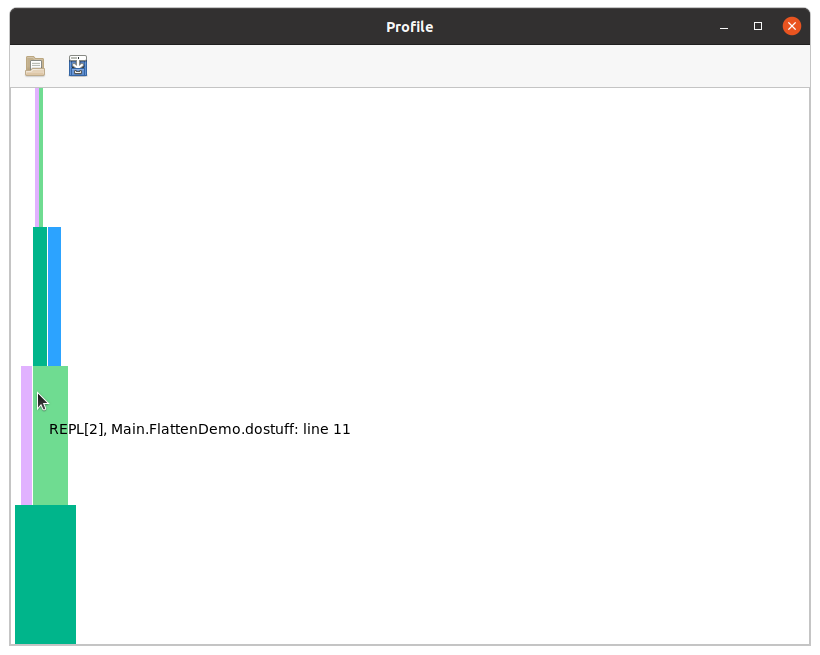
Users are encouraged to read the ProfileView documentation to understand how to interpret this, but briefly:
the horizontal axis is time (wide boxes take longer than narrow ones), the vertical axis is call depth
hovering over a box displays the method that was inferred
left-clicking on a box causes the full MethodInstance to be printed in your REPL session
right-clicking on a box opens the corresponding method in your editor (you must have
ENV["EDITOR"]configured appropriately for this to work)ctrl-click can be used to zoom in (you can do rubber band selection or zoom in/zoom out)
empty horizontal spaces correspond to activities other than type-inference; in this case, the relatively narrow flame followed by a lot of empty space indicates that all the type inference happened at the beginning and accounted for only a small fraction of the total time.
You can explore this flamegraph and compare it to the output from print_tree.
In less trivial examples, these flame graphs may look more interesting:
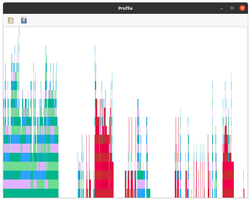
Here, the red boxes correspond to MethodInstances which cannot be "naturally" precompiled. This occurs when the method is owned by one module but the argument types are from another unrelated module. We'll see how to deal with these in later installments.
You also see breaks in the flamegraph. During these periods, code generation and runtime create new objects and then call methods on those objects; if one of those calls requires a fresh entrance into inference, that triggers the creation of a new flame. Hence, the number of distinct flames (which is just equal to length(tinf.children)) gives you a rough indication of how frequently the chains of inference were broken. This can be caused by type instability, separate top-level calls from the REPL during @snoopi_deep, calls to eval in your code, or some other cause for Julia to start running type inference.
PProf.jl
julia> fg = flamegraph(tinf)
Node(FlameGraphs.NodeData(ROOT() at typeinfer.jl:75, 0x00, 0:10080857))

julia> using PProf

julia> pprof(fg)
Serving web UI on http://localhost:57599
For a detailed walkthrough of how to use PProf, see the PProf.jl README and, for a more complete guide, the google/pprof web interface README.
We have found the most useful views for inspecting an inference profile to be the /flamegraph and /source views. If you navigate to the Flamegraph view, via VIEW -> Flame Graph, this is what you should see:
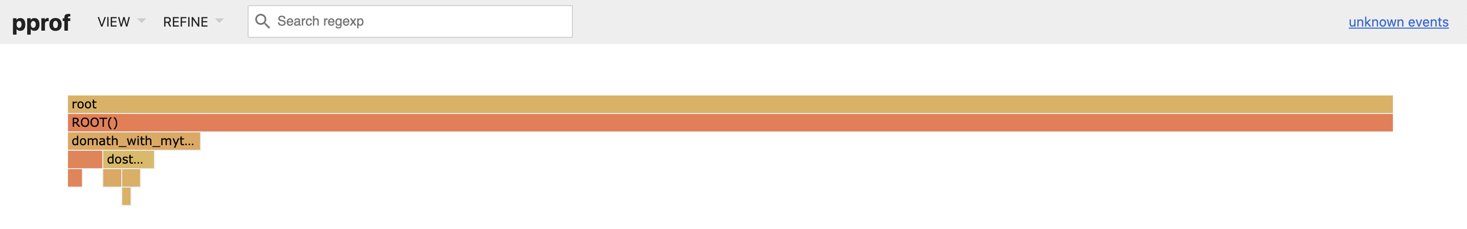
Of course, as above, in this example inference was only a small part of the total time. You can zoom-in on nodes by clicking on them, and hovering will display their full text and time. The nicest way to expand just the inference time is to filter out the non-inference time by "hiding" the ROOT() node. To do this, type ROOT() in the Search regexp bar and click REFINE -> Hide, or add ?h=ROOT to the URL. This works well if there are several top-level calls to inference, as discussed below. One benefit of hiding and filtering via the Search bar is that the percentages for all nodes will be recomputed as a percentage of the new total.
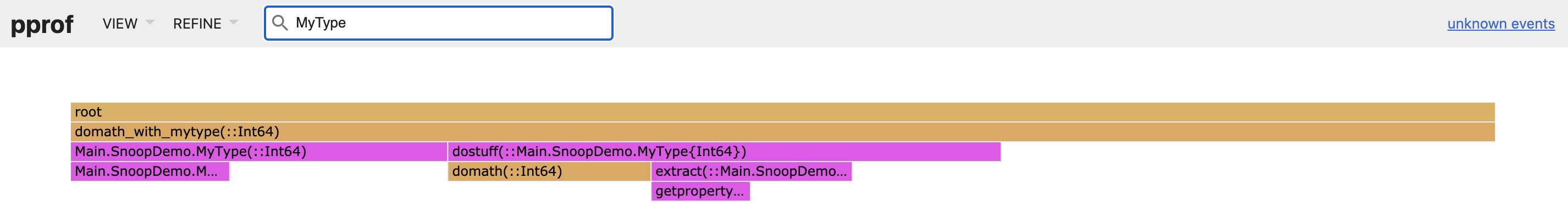
Typing values into the search bar (without pressing enter) will highlight them in the graph, as displayed in the following image, and pressing enter will filter the graph to only contain paths that match your search. These tools can be used to identify small functions that show up often, contributing large amounts of time when aggregated together.
Here's a screenshot of the Top view, again with ROOT() hidden (/top?h=ROOT()):

More details about using PProf are outside the scope of this post, but here are some things to keep in mind:
Sibling frames in pprof are not ordered by time, they are ordered alphabetically.
ProfileView, above, is a much better tool for understanding what occurred when during a computation.PProf is excellent for interactively exploring (potentially very large) profiles. It provides good high-level summary of the biggest offenders, and includes many tools for understanding their details, including the
sourceview,topview, and filtering.You can export profiles to a file via the
out=parameter topprof(), which are entirely self-contained and can be shared with collaborators for them to view with PProf.
Elementary analysis: flatten and accumulate_by_source
As our last step for this post, let's extract the data as a list:
julia> flatten(tinf)
10-element Vector{SnoopCompileCore.InferenceTiming}:
 InferenceTiming: 0.000034/0.000034 on InferenceFrameInfo for getproperty(::Main.SnoopDemo.MyType{Int64}, x::Symbol)
 InferenceTiming: 0.000045/0.000045 on InferenceFrameInfo for getproperty(::Main.SnoopDemo.MyType{Int64}, ::Symbol)
 InferenceTiming: 0.000071/0.000071 on InferenceFrameInfo for Main.SnoopDemo.MyType(::Int64)
 InferenceTiming: 0.000083/0.000161 on InferenceFrameInfo for Main.SnoopDemo.extract(::Main.SnoopDemo.MyType{Int64})
 InferenceTiming: 0.000122/0.000453 on InferenceFrameInfo for Main.SnoopDemo.dostuff(::Main.SnoopDemo.MyType{Int64})
 InferenceTiming: 0.000122/0.000254 on InferenceFrameInfo for Main.SnoopDemo.MyType(::Int64)
 InferenceTiming: 0.000132/0.000132 on InferenceFrameInfo for Main.SnoopDemo.MyType{Int64}(::Int64)
 InferenceTiming: 0.000170/0.000170 on InferenceFrameInfo for Main.SnoopDemo.domath(::Int64)
 InferenceTiming: 0.000355/0.001133 on InferenceFrameInfo for Main.SnoopDemo.domath_with_mytype(::Int64)
 InferenceTiming: 0.009382/0.010515 on InferenceFrameInfo for Core.Compiler.Timings.ROOT()
By default, this orders the nodes by exclusive time, but flatten(tinf; sortby=inclusive) allows you to sort by inclusive time. Finally, flatten(tinf; sortby=nothing) returns the nodes in the order in which they were inferred.
Sometimes, you might infer the same method for many different specific argument types, and sometimes you might want to get a sense of the aggregate cost:
julia> accumulate_by_source(flatten(tinf))
8-element Vector{Tuple{Float64, Union{Method, Core.MethodInstance}}}:
 (7.838100000000001e-5, getproperty(x, f::Symbol) in Base at Base.jl:33)
 (8.2955e-5, extract(y::Main.SnoopDemo.MyType) in Main.SnoopDemo at REPL[1]:4)
 (0.000121738, dostuff(y) in Main.SnoopDemo at REPL[1]:11)
 (0.000132328, Main.SnoopDemo.MyType{T}(x) where T in Main.SnoopDemo at REPL[1]:2)
 (0.000170205, domath(x) in Main.SnoopDemo at REPL[1]:6)
 (0.000193107, Main.SnoopDemo.MyType(x::T) where T in Main.SnoopDemo at REPL[1]:2)
 (0.000354527, domath_with_mytype(x) in Main.SnoopDemo at REPL[1]:13)
 (0.009381595, ROOT() in Core.Compiler.Timings at compiler/typeinfer.jl:75)
This shows the cost of each Method, summing across all specific MethodInstances.
Summary
The tools described here permit a new level of insight into where type inference is spending its time. Sometimes, this information alone is enough to show you how to change your code to reduce latency. However, most efforts at latency reduction will probably leverage additional tools that help identify the main opportunities for intervention. These tools will be described in future posts.