Knowing where you are: custom array indices in Julia

Arrays are a crucial component of any programming language, particularly for a data-oriented language like Julia. Arrays store values according to their location: in Julia, given a two-dimensional array A, the expression A[1,3] returns the value stored at a location known as (1,3). If, for example, A stores Float64 numbers, the value returned by this expression will be a single Float64 number.

Julia's arrays conventionally start numbering their axes with 1, meaning that the first element of a one-dimensional array a is a[1]. The choice of 1 vs. 0 seems to generate a certain amount of discussion. A fairly recent addition to the Julia landscape is the ability to define arrays that start with an arbitrary index. The purpose of this blog post is to describe why this might be interesting. This is really a "user-oriented" blog post, hinting at some of the ways this new feature can make your life simpler. For developers who want to write code that supports arrays with arbitrary indices, see this documentation page.

Why should we care which indices an array has? A first example

Sometimes arrays are used as simple lists, in which case the indices may not matter to you. But in other cases, arrays are used as a discrete representation of a continuous quantity (e.g., values defined over space or time), and in such cases the array indices correspond to "location" in a way that may be meaningful.

As a simple example, consider the process of rotating an image:

img	img_rotated

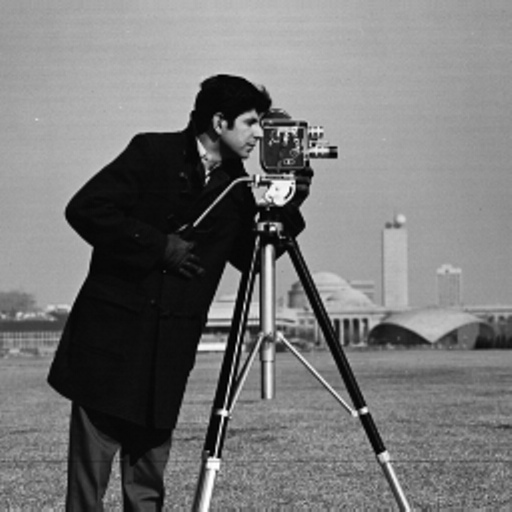Many languages provide functions for rotating an image; in Julia, you can do this with the warp function defined in ImageTransformations.

Things get a little more "interesting" when you want to compare pixels in the rotated image to those of the original image. How, exactly, do these pixels match up? In other words, for a location img[i,j], what is the corresponding i′,j′ location in img_rotated? In many languages, figuring out these types of geometric alignments may not be a simple task; it's no exaggeration to say that in complex situations (e.g., a three-dimensional image with a complex spatial deformation) that one can spend a day or more figuring out exactly how pixels/voxels in two images are supposed to be compared.

Why is this such a hard problem? The core problem is that, in most cases, the language is essentially "lying" to you about the location of pixels: if arrays always start indexing at 1 along any given axis, the array indices don't really correspond to an absolute spatial location. An index of 1 means "first index" rather than "spatial location 1."

So to fix this in Julia, starting with version 0.5 we support arrays with indices that don't start with 1. Let's illustrate this by specifying that we want the above rotation to be around a point in the head of the cameraman. Let's load the image:

julia> using Images, TestImages

julia> img = testimage("cameraman");

julia> summary(img)
"512×512 Array{Gray{N0f8},2}"

summary shows that img is a grayscale image indexed over the ranges 1:512×1:512. Using any of several approaches (e.g., ImageView and paying attention to the status bar to get the mouse pointer location), we can learn that the point (y=126, x=251) is in the head of the cameraman. Consequently, let's define a rotation around this point:

julia> using Rotations, CoordinateTransformations

julia> tfm = Translation(125,250) ∘ LinearMap(RotMatrix(pi/6)) ∘ Translation(-125,-250)
AffineMap([0.866025 -0.5; 0.5 0.866025], [141.747, -29.0064])

This defines tfm as the composition of a translation (shifting the head to the origin) followed by a rotation, and then translating back. (You can get the composition operator ∘ by typing \circ and then hitting TAB.) If we apply this transformation to the image, we get an interesting result:

julia> img_rotated = warp(img, tfm);

julia> summary(img_rotated)
"-107:592×-160:539 OffsetArray{Gray{N0f8},2}"

Perhaps surprisingly, img_rotated is indexed over the range -107:592×-160:539, meaning that we access the upper left corner by img_rotated[-107,-160] and the lower right corner by img_rotated[592,539]. It's not hard to see why these numbers arise, if we see how the corners of img are transformed by tfm:

julia> using StaticArrays

julia> itfm = inv(tfm)
AffineMap([0.866025 0.5; -0.5 0.866025], [-108.253, 95.9936])

julia> itfm(SVector(1,1))
2-element SVector{2,Float64}:
 -106.887
   96.3597

julia> itfm(SVector(512,1))
2-element SVector{2,Float64}:
  335.652
 -159.14

julia> itfm(SVector(1,512))
2-element SVector{2,Float64}:
 148.613
 538.899

julia> itfm(SVector(512,512))
2-element SVector{2,Float64}:
 591.152
 283.399

This makes it apparent that the output's indices span the region of the transformed coordinates.

The fact that the output preserves the coordinates makes it trivial to compare the images:

julia> cv = colorview(RGB, paddedviews(0, img, img_rotated, img)...)

paddedviews(0, arrays...) pads input arrays with 0, as needed, to give them all the same indices, and colorview(RGB, r, g, b) inserts the grayscale images r, g, and b into the red, green, and blue channels respectively. If we visualize cv, we see the following:

around image center	around head (cv)

The image on the left is for reference, showing what a rotation around the image center would look like when properly aligned. The image on the right corresponds to the steps taken above, and indeed confirms that the rotation is around the head. Alternatively, we can focus on the overlapping portions of these images like this:

julia> inds = map(intersect, indices(img), indices(img_rotated))
(1:512, 1:512)

julia> imgi = img[inds...];

julia> imgri = img_rotated[inds...];

so that colorview(RGB, imgi, imgri, imgi) displays as

cameraman_interior

Since the indices of the pixels encode absolute spatial location, it's trivial to keep track of how different pixels align: pixel i,j in one image corresponds to pixel i,j in the other. This is true even if our coordinate transformation were far more complicated than a simple rotation.

Having motivated why this might be useful, let's take a step back and walk through array indices a bit more systematically.

A systematic introduction to arrays with arbitrary indices

In Julia, if we define an array

julia> A = collect(reshape(1:30, 5, 6))
5×6 Array{Int64,2}:
 1   6  11  16  21  26
 2   7  12  17  22  27
 3   8  13  18  23  28
 4   9  14  19  24  29
 5  10  15  20  25  30

then we can refer to a rectangular region like this:

julia> B = A[1:3, 1:4]
3×4 Array{Int64,2}:
 1  6  11  16
 2  7  12  17
 3  8  13  18

For certain applications, one negative to extracting blocks is that there is no record indicating where the new block originated from:

julia> B2 = A[2:4, 1:4]
3×4 Array{Int64,2}:
 2  7  12  17
 3  8  13  18
 4  9  14  19

julia> B2[1,1]
2

So B2[1,1] corresponds to A[2,1], despite the fact that, as measured by their indices, these are not the same location.

To maintain consistent "naming" of our indices, let's use the OffsetArrays package:

julia> using OffsetArrays

julia> B3 = OffsetArray(A[2:4, 1:4], 2:4, 1:4)  
# wrap the snipped-out piece in an OffsetArray
OffsetArrays.OffsetArray{Int64,2,Array{Int64,2}} with indices 2:4×1:4:
 2  7  12  17
 3  8  13  18
 4  9  14  19

julia> B3[3,4]
18

julia> A[3,4]
18

So the indices in B3 match those of A. Indeed, B3 doesn't even have an element "named" (1,1):

julia> B3[1,1]
ERROR: BoundsError: attempt to access OffsetArrays.OffsetArray{Int64,2,Array{Int64,2}}
 with indices 2:4×1:4 at index [1, 1]
Stacktrace:
 [1] throw_boundserror(::OffsetArrays.OffsetArray{Int64,2,Array{Int64,2}}, ::Tuple{Int64,Int64}) at ./abstractarray.jl:426
 [2] checkbounds at ./abstractarray.jl:355 [inlined]
 [3] getindex(::OffsetArrays.OffsetArray{Int64,2,Array{Int64,2}}, ::Int64, ::Int64) at /home/tim/.julia/v0.6/OffsetArrays/src/OffsetArrays.jl:89

In this case we created B3 by explicitly "wrapping" the extracted array inside a type that allows you to supply custom indices. (You can retrieve just the extracted portion with parent(B3).) We could do the same thing by adjusting the indices instead:

julia> using IdentityRanges

julia> ind1, ind2 = IdentityRange(2:4), IdentityRange(1:4)
(IdentityRange(2:4), IdentityRange(1:4))

An IdentityRange is a range with indices that match its values, r[i] == i. (ind1, ind2 = OffsetArray(2:4, 2:4), OffsetArray(1:4, 1:4) would be functionally equivalent.) Let's use ind1 and ind2 to snip out the region of the array:

julia> B4 = A[ind1, ind2]
OffsetArrays.OffsetArray{Int64,2,Array{Int64,2}} with indices 2:4×1:4:
 2  7  12  17
 3  8  13  18
 4  9  14  19

julia> B4[3,4]
18

This implements a simple rule of composition:

If `C = A[ind1, ind2]`, then `C[i, j] == A[ind1[i], ind2[j]]`

Consequently, if your indices have their own unconventional indices, they will be propagated forward to the next stage.

This technique can also be used to create a "view":

julia> V = view(A, ind1, ind2)
SubArray{Int64,2,Array{Int64,2},Tuple{IdentityRanges.IdentityRange{Int64},IdentityRanges.IdentityRange{Int64}},false} with indices 2:4×1:4:
 2  7  12  17
 3  8  13  18
 4  9  14  19

julia> V[3,4]
18

julia> V[1,1]
ERROR: BoundsError: attempt to access SubArray{Int64,2,Array{Int64,2},Tuple{IdentityRanges.IdentityRange{Int64},IdentityRanges.IdentityRange{Int64}},false} with indices 2:4×1:4 at index [1, 1]
Stacktrace:
 [1] throw_boundserror(::SubArray{Int64,2,Array{Int64,2},Tuple{IdentityRanges.IdentityRange{Int64},IdentityRanges.IdentityRange{Int64}},false}, ::Tuple{Int64,Int64}) at ./abstractarray.jl:426
 [2] checkbounds at ./abstractarray.jl:355 [inlined]
 [3] getindex(::SubArray{Int64,2,Array{Int64,2},Tuple{IdentityRanges.IdentityRange{Int64},IdentityRanges.IdentityRange{Int64}},false}, ::Int64, ::Int64) at ./subarray.jl:184

Note that this object is a conventional SubArray (it's not an OffsetArray), but because it was passed IdentityRange indices it preserves the indices of the indices.

A second application: array/image filtering (convolution)

As illustrated above for the image rotation example, a recent release (v0.6.0) of the Images package put both the power and responsibility for dealing with arrays with custom indices into the hands of users. One of the key functions in this package is imfilter which can be used to smooth or otherwise "filter" arrays. The idea is that starting from an array A, each local neighborhood is weighted by a "kernel" kern, producing an output value according to the following formula:

F[I] = \sum_J A[I+J] kern[J]

This is the formula for correlation; the formula for another operation, convolution, is very similar.

Let's start with a trivial example: let's filter with a "delta function" kernel, meaning it has value 1 at location 0 and is zero everywhere else. According to the correlation formula, because kern[J] is 1 at J==0, this should simply give us a copy of our original array:

julia> using Images

julia> imfilter(1:8, [1])
WARNING: assuming that the origin is at the center of the kernel;
to avoid this warning, call `centered(kernel)` or use an OffsetArray
Stacktrace:
 [1] depwarn(::String, ::Symbol) at ./deprecated.jl:64
 [2] _kernelshift at /home/tim/.julia/v0.6/ImageFiltering/src/imfilter.jl:1049 [inlined]
 [3] kernelshift at /home/tim/.julia/v0.6/ImageFiltering/src/imfilter.jl:1046 [inlined]
 [4] factorkernel(::Array{Int64,1}) at /home/tim/.julia/v0.6/ImageFiltering/src/imfilter.jl:1016
 [5] imfilter at /home/tim/.julia/v0.6/ImageFiltering/src/imfilter.jl:10 [inlined]
 [6] imfilter(::UnitRange{Int64}, ::Array{Int64,1}) at /home/tim/.julia/v0.6/ImageFiltering/src/imfilter.jl:5
 [7] eval(::Module, ::Any) at ./boot.jl:235
 [8] eval_user_input(::Any, ::Base.REPL.REPLBackend) at ./REPL.jl:66
 [9] macro expansion at ./REPL.jl:97 [inlined]
 [10] (::Base.REPL.##1#2{Base.REPL.REPLBackend})() at ./event.jl:73
while loading no file, in expression starting on line 0
8-element Array{Int64,1}:
 1
 2
 3
 4
 5
 6
 7
 8

The warning is telling you that Images decided to make a guess about your intention, that the kernel [1] was intended to be centered around zero. You can suppress the warning by explicitly passing the following kernel instead:

julia> kern = centered([1])
OffsetArrays.OffsetArray{Int64,1,Array{Int64,1}} with indices 0:0:
 1

julia> kern[0]
1

julia> kern[1]
ERROR: BoundsError: attempt to access OffsetArrays.OffsetArray{Int64,1,Array{Int64,1}} with indices 0:0 at index [1]
Stacktrace:
 [1] throw_boundserror(::OffsetArrays.OffsetArray{Int64,1,Array{Int64,1}}, ::Tuple{Int64}) at ./abstractarray.jl:426
 [2] checkbounds at ./abstractarray.jl:355 [inlined]
 [3] getindex(::OffsetArrays.OffsetArray{Int64,1,Array{Int64,1}}, ::Int64) at /home/tim/.julia/v0.6/OffsetArrays/src/OffsetArrays.jl:94

By using an OffsetArray you have clearly specified your intended indices for kern.

This can be used to shift an image in the following way (by default, imfilter returns its results over the same domain as the input):

julia> kern2 = OffsetArray([1], 2:2)  # a delta function centered at 2
OffsetArrays.OffsetArray{Int64,1,Array{Int64,1}} with indices 2:2:
 1

julia> imfilter(1:8, kern2, Fill(0))  # pad the edges of the input with 0
8-element Array{Int64,1}:
 3
 4
 5
 6
 7
 8
 0
 0

julia> kern3 = OffsetArray([1], -5:-5)   # a delta function centered at -5
OffsetArrays.OffsetArray{Int64,1,Array{Int64,1}} with indices -5:-5:
 1

julia> imfilter(1:8, kern3, Fill(0))
8-element Array{Int64,1}:
 0
 0
 0
 0
 0
 1
 2
 3

These are all illustrated in the following figure:

deltafunctions

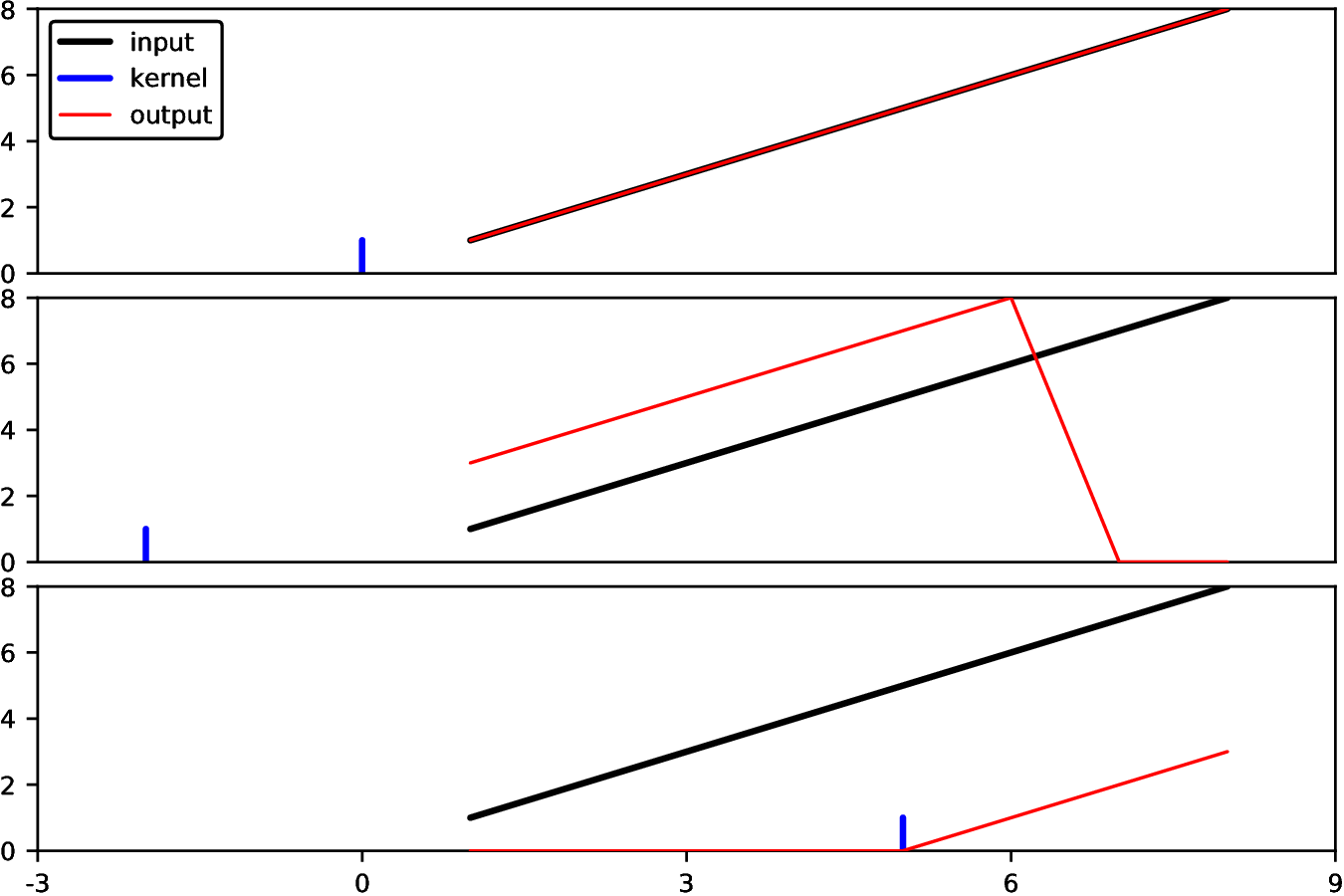
In this figure, we plotted the kernel as if it were at the location corresponding to convolution rather than correlation.

In other programming languages, when filtering with a kernel that has an even number of elements, it can be difficult to remember which of the two middle elements corresponds to the origin. In Julia, that's not an issue, because you can make that choice for yourself:

julia> kern = OffsetArray([0.5,0.5], 0:1)
OffsetArrays.OffsetArray{Float64,1,Array{Float64,1}} with indices 0:1:
 0.5
 0.5

julia> imfilter(1:8, kern, Fill(0))
8-element Array{Float64,1}:
 1.5
 2.5
 3.5
 4.5
 5.5
 6.5
 7.5
 4.0

julia> kern = OffsetArray([0.5,0.5], -1:0)
OffsetArrays.OffsetArray{Float64,1,Array{Float64,1}} with indices -1:0:
 0.5
 0.5

julia> imfilter(1:8, kern, Fill(0))
8-element Array{Float64,1}:
 0.5
 1.5
 2.5
 3.5
 4.5
 5.5
 6.5
 7.5

Likewise, sometimes we might have an application where we simply can't handle the edges properly, and we wish to discard them. For example, consider the following quadratic function:

julia> a = [(i-3)^2 for i = 1:9]  # a quadratic function
9-element Array{Int64,1}:
  4
  1
  0
  1
  4
  9
 16
 25
 36

julia> imfilter(a, Kernel.Laplacian((true,)))
9-element Array{Int64,1}:
  -3
   2
   2
   2
   2
   2
   2
   2
 -11

Those weird values on the edges (for which there is no padding that will "extrapolate" the quadratic) might cause problems. Consequently, let's only extract the values that are well-defined, meaning that all inputs to the correlation formula have explicitly-assigned values:

julia> imfilter(a, Kernel.Laplacian((true,)), Inner())
OffsetArrays.OffsetArray{Int64,1,Array{Int64,1}} with indices 2:8:
 2
 2
 2
 2
 2
 2
 2

Notice that in this case, it returned an OffsetArray so that the values in the result align properly with the original array.

A final application: Fourier transforms

There are many more things you can do with custom indices. As one last illustration, consider the Discrete Fourier Transform, which is defined on a periodic domain. Typically, it's rather difficult to emulate a periodic domain with arrays, because arrays have finite size. However, it's possible to define indexing objects which possess periodic behavior. Here we use the FFTViews package, demonstrating the technique on a simple sinusoid:

julia> using FFTViews

julia> a = [sin(2π*x)+0.1 for x in linspace(0,1,16)];

julia> afft = FFTView(fft(a))
FFTViews.FFTView{Complex{Float64},1,Array{Complex{Float64},1}} with indices FFTViews.URange(0,15):
       1.6+0.0im
     1.498-7.53098im
 -0.288537+0.69659im
 -0.236488+0.35393im
 -0.222614+0.222614im
 -0.216932+0.14495im
 -0.214217+0.0887316im
 -0.212937+0.0423558im
 -0.212557+0.0im
 -0.212937-0.0423558im
 -0.214217-0.0887316im
 -0.216932-0.14495im
 -0.222614-0.222614im
 -0.236488-0.35393im
 -0.288537-0.69659im
     1.498+7.53098im

Now, as every student of Fourier transforms learns, the 0-frequency bin holds the sum of the values in a:

julia> afft[0]
1.6000000000000003 + 0.0im

Since the mean of a sinusoid is zero, this is (within roundoff error) 16*0.1 = 1.6.

We can also check the amplitude at the Fourier-peak, and explore the periodicity of the result:

julia> afft[1]
1.4980046017247872 - 7.53097769363728im

julia> afft[-1]      # negative frequencies are OK
1.4980046017247872 + 7.53097769363728im

julia> afft[64+1]    # look Ma, it's periodic!
1.4980046017247872 - 7.53097769363728im

julia> length(indices(afft,1))   # but we still know how big it is
16

Given the periodicity of afft, the commonly-used fftshift function (e.g., fftshift(fft(a))) can be replaced by afft[-8:7]. While very simple, these techniques make it surprisingly more pleasant to deal with what can sometimes become complex and error-prone index gymnastics.

Summary: a user's perspective

This has only scratched the surface of what's possible with custom indices. In the opinion of the author, their main advantage is that they can increase the clarity of code by ensuring that "names" (indices) can be endowed with absolute meaning, rather than always being "referenced to whatever the first element of this particular array happens to encode."

There is quite a lot of code that hasn't yet properly accounted for the possibility of custom indices — surely, some of it written by the author of this post! So users should be prepared for the possibility that exploiting custom indices will trigger errors in base Julia or in packages. Rather than giving up, users are encouraged to report such errors as issues, as this is the only way that custom indices will, over the course of time, have solid support.

Summary: a developer's perspective

For some algorithms, there appears to be little reason to ever use arrays with anything but 1-based indices; in such cases, there may be no reason to modify existing code. But if your code has a "spatial" interpretation–where location has meaning–then you just might want to give the new facilities a try.

In transitioning existing code, the author of this post has observed the following tendencies:

algorithms that exploit custom indices are sometimes simpler to understand than their "1-locked" counterparts;
if you're porting old code to support custom indices, there's some bad news: if you had to think carefully about the indexing the first time you wrote it, it usually requires significant investment to re-think the indexing, even if the end result is somewhat simpler.
even when a specific algorithm might gain little advantage from supporting arbitrary indices, writing code that is "indices aware" from the beginning is often no harder than writing algorithms that implicitly assume indexing starts at 1.

Developers are referred to Julia's documentation for further guidance.