This post will demonstrate how to set up and simulate a model of a swimming dogfish shark using Julia and WaterLily.jl. This post is adapted from a Pluto notebook that you can get here.
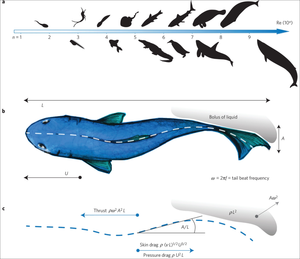
using WaterLily, StaticArrays, PlutoUI, Interpolations, Plots, ImagesWe'll use a simple model of the shark based on Lighthill's pioneering paper on the swimming of slender fish. It focuses on the "backbone" of the fish; idealizing the shape as a thickness distribution on either side of the center, and the motion as a lateral ("side-to-side") traveling wave. Amazingly, this simple approach provides insight across a huge range of a swimming animals as illustrated in the image below. Image credit: Gazzola et al, Nature 2014
We'll define the thickness and motion distributions using interpolate to fit splines through a few points.
fit = y -> scale(
        interpolate(y, BSpline(Quadratic(Line(OnGrid())))),
        range(0,1,length=length(y))
    )
Here is an image of the dogfish shark we will model. Image credit: Shark Trust.
url2 = "https://pterosaurheresies.files.wordpress.com/2020/01/squalus-acanthias-invivo588.jpg"
filename2 = download(url2)
dogfish = load(filename2)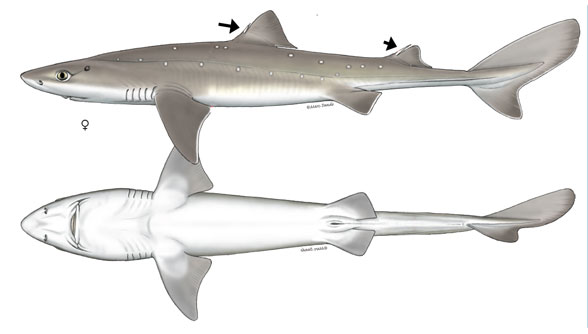
The bottom view shows the outline we're interested in, and adding a few points along the length defines the thickness distribution function thk.
plot(dogfish)
nose, len = (30,224), 500
width = [0.02, 0.07, 0.06, 0.048, 0.03, 0.019, 0.01]
scatter!(
	nose[1] .+ len .* range(0, 1, length=length(width)),
	nose[2] .- len .* width, color=:blue, legend=false)
thk = fit(width)
x = 0:0.01:1
plot!(
	nose[1] .+ len .* x,
	[nose[2] .- len .* thk.(x), nose[2] .+ len .* thk.(x)],
	color=:blue)
Looking at videos of swimming dogfish, we can see a couple general features
The motion of the front half of the body has a small amplitude (around 20% of the tail). This sets the amplitude envelope for the traveling wave.
envelope = [0.2,0.21,0.23,0.4,0.88,1.0]
amp = fit(envelope)
The wavelength of the traveling wave is a bit longer than the body length
In the code below, you can change the value of to control the wavelength of the traveling wave to see the impact it has on the backbone over the motion cycle.
λ = 1.4
scatter(0:0.2:1, envelope)
colors = palette(:cyclic_wrwbw_40_90_c42_n256)
for t in 1/12:1/12:1
	plot!(x, amp.(x) .* sin.(2π/λ * x .- 2π*t),
		  color=colors[floor(Int,t*256)])
end
plot!(ylim=(-1.4,1.4), legend=false)
Now the thickness and motion are defined, but how will we apply these to a fluid simulation? WaterLily uses an immersed boundary method and automatic differentiation to embed a body into the flow. The upshot is that we don't need to do any meshing; all we need is a signed distance function (SDF) to the surface.
Let's start by defining the SDF to the "backbone", which is a line segment from . See this great video from Inigo Quilez for a derivation of this sdf.. The plot below shows the sdf and the zero contour, which is ... just a line segment.
Simple adjustments to the SDF give us more control of the shape and position. By shifting the y offset as y = y-shift, we can move the body laterally. And by subtracting a thickness from the distance as sdf = sdf-thickness, we can give the line some width. This is all we need to model the shark.
shift = 0.5
T = 0.5

function segment_sdf(x, y)
	s = clamp(x, 0, 1)          # distance along the segment
	y = y - shift               # shift laterally
	sdf = √sum(abs2, (x-s, y))  # line segment SDF
	return sdf - T * thk(s)     # subtract thickness
end

grid = -1:0.05:2
contourf(grid, grid, segment_sdf, clim=(-1,2), linewidth=0)
contour!(grid, grid, segment_sdf, levels=[0], color=:black)  # zero contour
With the basic SDF tested out, we are ready to set up the WaterLily simulation using the function fish defined below:
The functions thk is passed in to create the sdf and the function amp is passed in to create the traveling wave map.
The only numerical parameter passed into fish is the length of the fish L measured in computational cells. This sets the resolution of the simulation and the size of the fluid arrays.
The other parameters are the tail amplitude A as a fraction of the length, the Stouhal number which sets the motion frequency ω, and the Reynolds number which sets the fluid viscosity ν.
function fish(thk, amp, k=5.3; L=2^6, A=0.1, St=0.3, Re=1e4)
	# fraction along fish length
	s(x) = clamp(x[1]/L, 0, 1)

	# fish geometry: thickened line SDF
	sdf(x,t) = √sum(abs2, x - L * SVector(s(x), 0.)) - L * thk(s(x))

	# fish motion: travelling wave
	U = 1
	ω = 2π * St * U/(2A * L)
	function map(x, t)
		xc = x .- L # shift origin
		return xc - SVector(0., A * L * amp(s(xc)) * sin(k*s(xc)-ω*t))
	end

	# make the fish simulation
	return Simulation((4L+2,2L+2), [U,0.], L;
						ν=U*L/Re, body=AutoBody(sdf,map))
end

# Create the swimming shark
L,A,St = 3*2^5,0.1,0.3
swimmer = fish(thk, amp; L, A, St);

# Save a time span for one swimming cycle
period = 2A/St
cycle = range(0, 23/24*period, length=24)
We can test our geometry by plotting the immersed boundary function μ₀; which equals 1 in the fluid and 0 in the body.
@gif for t ∈ cycle
	measure!(swimmer, t*swimmer.L/swimmer.U)
	contour(swimmer.flow.μ₀[:,:,1]',
			aspect_ratio=:equal, legend=false, border=:none)
end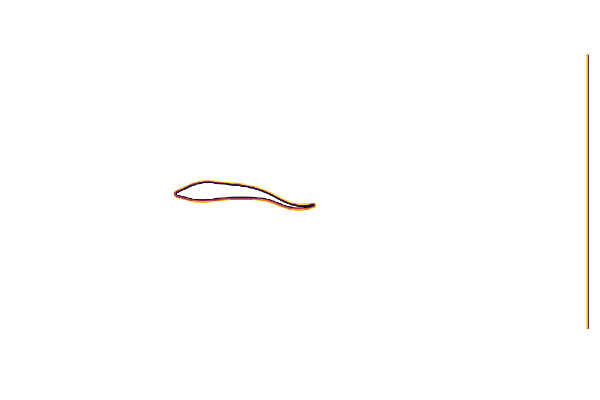
That animation of the motion looks great, so we are ready to run the flow simulator!
The sim_step!(sim, t, remeasure=true) function runs the simulator up to time t, remeasuring the body position every time step. (remeasure=false by default since it takes a little extra computational time and isn't needed for statics geometries.)
# run the simulation a few cycles (this takes few seconds)
sim_step!(swimmer, 10, remeasure=true)
sim_time(swimmer)
The simulation has now run forward in time, but there are no visualizations or measurements by default.
To see what is going on, lets make a gif of the vorticity ω=curl(u) to visualize the vortices in the wake of the shark. This requires simulating a cycle of motion, and computing the curl at all the points @inside the simulation.
# plot the vorcity ω=curl(u) scaled by the body length L and flow speed U
function plot_vorticity(sim)
	@inside sim.flow.σ[I] = WaterLily.curl(3, I, sim.flow.u) * sim.L / sim.U
	contourf(sim.flow.σ',
			 color=palette(:BuGn), clims=(-10, 10), linewidth=0,
			 aspect_ratio=:equal, legend=false, border=:none)
end

# make a gif over a swimming cycle
@gif for t ∈ sim_time(swimmer) .+ cycle
	sim_step!(swimmer, t, remeasure=true)
	plot_vorticity(swimmer)
end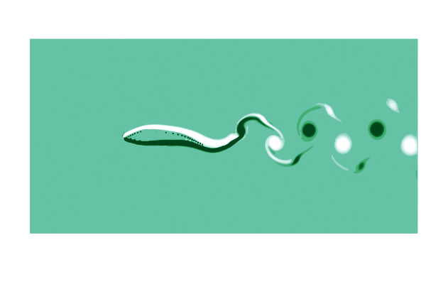
This is pretty (CFD does stand for Colorful Fluid Dynamics after all), but also tells us something important about the flow. Notice that there are no eddies coming off the body anywhere other than the tail! This is a sign of efficiency since energy is only used to create those trailing vortices.
We can dig in and get some quantitative measurements from the simulation as well. The function ∮nds takes a integral over the body surface. By passing in the pressure p, we can measure the thrust force and side force generated by the shark!
function get_force(sim, t)
	sim_step!(sim, t, remeasure=true)
	return WaterLily.∮nds(sim.flow.p, sim.body, t*sim.L/sim.U) ./ (0.5*sim.L*sim.U^2)
end
forces = [get_force(swimmer, t) for t ∈ sim_time(swimmer) .+ cycle]

scatter(cycle./period, [first.(forces), last.(forces)],
		labels=permutedims(["thrust", "side"]),
		xlabel="scaled time",
		ylabel="scaled force")
We can learn a lot from this simple plot. For example, the side-to-side force has the same frequency as the swimming motion itself while the thrust force has double the frequency, with a peak every time the tail passes through the centerline.
This simple model is a great start and it opens up a ton of avenues for improving the shark simulation and suggesting research questions:
The instantaneous net forces should be zero in a free swimming body! We could add reaction motions to our model to achieve this. Would the model shark swim in a straight line if we did this, or is a control-loop needed?
Real sharks are 3D (gasp!). While we could easily extend this approach using 2D splines, it will take much longer to simulate. Is there a way use GPUs to accelerate the simulations without completely changing the solver?
If we were going to make a bio-inspired robot of this shark, we will have constraints on the shape and motion and powering available. Can we use this framework to help optimize our robotic within it's constraints?
Below you can find links to all the packages used in this notebook. Happy Simulating!
Pluto.jl and PlutoUI.jl